# Kaiser window state

In this example, We introduce the preparation of Kaiser window state.&#x20;

### What is Kaiser window state

The state is defined as

$$
|\Psi\rangle := \frac{1}{\sqrt{\sum\_x |f(x)|^2}} \sum\_{x=0}^{N-1} f(x) |x\rangle
$$

where the amplitude is described by the Kaiser window function $$f(x) = \frac{I\_0(\beta \sqrt{1-x^2})}{I\_0 (\beta)}$$. Here, $$I\_0$$ is the zeroth modified Bessel function of the first kind. The Kaiser window function can be used in quantum phase estimation to boost the success probability without (coherently) calculating the median of several phase evaluations.&#x20;

### The equivalent problem in function approximation

One recent preprint Ref. [\[1\]](#reference) proposed a procedure for preparing Kaiser window state. It leverages the block encoding of the sine value of equally spaced sample points $$\sum\_x \sin(x/N)|x\rangle\langle x|$$. By applying quantum eigenvalue transformation on this block encoding, the Kaiser window state is prepared. Consequently, the problem is reduced to finding the phase factors generating the following function

$$
h(z) = f(\arcsin(z)) \propto I\_0(\beta \sqrt{1 - \arcsin^2(z)}).
$$

where $$z = \sin(x)$$ transforms the domain to $$z\in \[0,\sin(1)]$$.

### Setup parameters

```matlab
beta = 8; 
targ = @(x) besselj(0,1jbetasqrt(1-2asin(x).^2))/besselj(0,1jbeta);

deg = 100; 
delta = 0.01; 
opts.intervals = [0,sin(1)]; 
opts.objnorm = Inf; 
opts.epsil = 0.01; 
opts.npts = 500; 
opts.fscale = 0.98; % scaling factor for the infinity norm 
opts.isplot = true;

opts.maxiter = 100; 
opts.criteria = 1e-12; 
opts.useReal = true; 
opts.targetPre = true; 
opts.method = 'Newton';
```

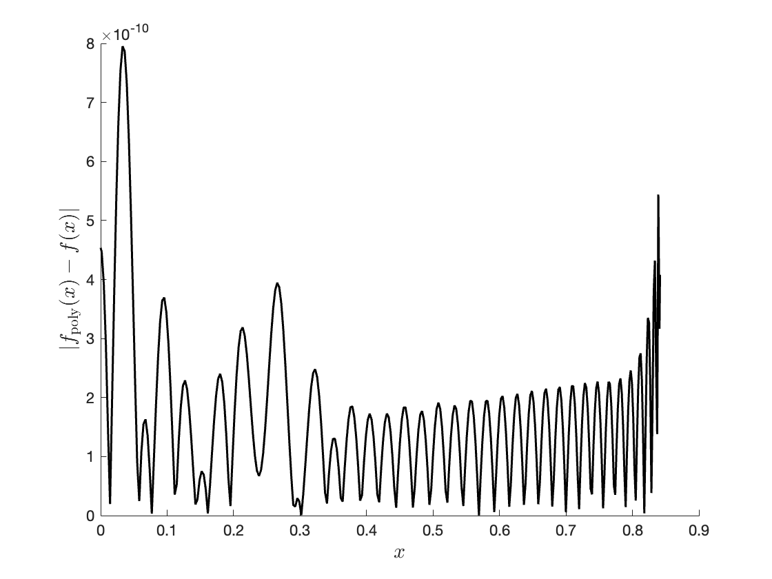
### Approximating the target function by polynomials

```matlab
coef_full=cvx_poly_coef(targ, deg, opts); 
parity = mod(deg, 2); 
% only keep coefficients with consistent parity
coef = coef_full(1+parity:2:end);
```

<div><figure><img src="https://40428858-files.gitbook.io/~/files/v0/b/gitbook-x-prod.appspot.com/o/spaces%2FznDlSgNqsJLx79OHu47P%2Fuploads%2FAsPUmA5DCjsqQj5N1Say%2Fkaiser_window_polynomial.png?alt=media&#x26;token=5094f62d-32ef-49b1-be7f-b24211e49350" alt=""><figcaption><p>Polynomial approximation of Kaiser window function</p></figcaption></figure> <figure><img src="https://40428858-files.gitbook.io/~/files/v0/b/gitbook-x-prod.appspot.com/o/spaces%2FznDlSgNqsJLx79OHu47P%2Fuploads%2FvLqnlViUA8vrMvgbFZFS%2Fkaiser_window_pointwise_error.png?alt=media&#x26;token=a2b143a1-92ca-46b8-ac8a-3f64055fb586" alt=""><figcaption><p>Polynomial approximation error</p></figcaption></figure></div>

### Solving phase factors by running the solver

```matlab
[phi_proc,out] = QSP_solver(coef,parity,opts);
```

### Verifying the solution

```matlab
xlist = linspace(0,sin(1),500)';
func = @(x) ChebyCoef2Func(x, coef, parity, true);
targ_value = targ(xlist);
func_value = func(xlist);
QSP_value = QSPGetEntry(xlist, phi_proc, out);
err= norm(QSP_value-func_value,Inf);
disp('The residual error is');
disp(err);

figure()
plot(xlist,QSP_value-func_value)
xlabel('$x$', 'Interpreter', 'latex')
ylabel('$g(x,\Phi^*)-f_\mathrm{poly}(x)$', 'Interpreter', 'latex')
```

<figure><img src="https://40428858-files.gitbook.io/~/files/v0/b/gitbook-x-prod.appspot.com/o/spaces%2FznDlSgNqsJLx79OHu47P%2Fuploads%2FSJcBo8Q4JOBR9jLpfPTe%2Fkaiser_window_qsp_error.png?alt=media&#x26;token=73dbd07d-fa3a-481f-9e55-36436d7143dd" alt="" width="563"><figcaption><p>The point-wise error of the solved phase factors.</p></figcaption></figure>

### Reference

1. McArdle, S., Gilyén, A., & Berta, M. (2022). Quantum state preparation without coherent arithmetic. *arXiv preprint arXiv:2210.14892*.

<details>

<summary>Output of the code</summary>

```
norm error = 7.95198e-10
max of solution = 0.98
iter          err
   1  +1.4954e-01 
   2  +3.1526e-02 
   3  +4.7426e-03 
   4  +2.2475e-04 
   5  +6.1800e-07 
   6  +4.7263e-12 
Stop criteria satisfied.
The residual error is
   9.1038e-15
```

</details>
