# Gaussian state

In this example, We introduce the preparation of Gaussian state.&#x20;

### What is Gaussian state

Gaussian state is a $$n$$-qubit quantum state defined as

$$
|\Psi\rangle := \frac{1}{\sqrt{\sum\_x |f(x)|^2}} \sum\_{x=0}^{N-1} f(x) |x\rangle.
$$

where $$f(x) = \exp(-\beta x^2 / 2)$$ is the Gaussian function. Gaussian state is ubiquitous in the application of quantum algorithms in quantum chemistry, simulating quantum field theory, and quantum finance.

### The equivalent problem in function approximation

One recent preprint Ref. [\[1\]](#reference) proposed a procedure for preparing Gaussian state. It leverages the block encoding of the sine value of equally spaced sample points $$\sum\_x \sin(x/N)|x\rangle\langle x|$$. By applying quantum eigenvalue transformation on this block encoding, the Gaussian state is prepared. Consequently, the problem is reduced to finding the phase factors generating the following function

$$
h(z) = f(\arcsin(z)) \propto \exp(-\beta \arcsin^2(x) / 2).
$$

where $$z = \sin(x)$$ transforms the domain to $$z\in \[0,\sin(1)]$$.

### Setup parameters

```matlab
beta = 100;
targ = @(x) exp(-beta/2 *asin(x).^2);

deg = 100;
opts.intervals=[0,sin(1)];
opts.objnorm = Inf;
opts.epsil = 0.01;
opts.npts = 500;
opts.fscale = 0.99;
opts.isplot=true;

opts.maxiter = 100;
opts.criteria = 1e-12;
opts.useReal = true;
opts.targetPre = true;
opts.method = 'LBFGS';
```

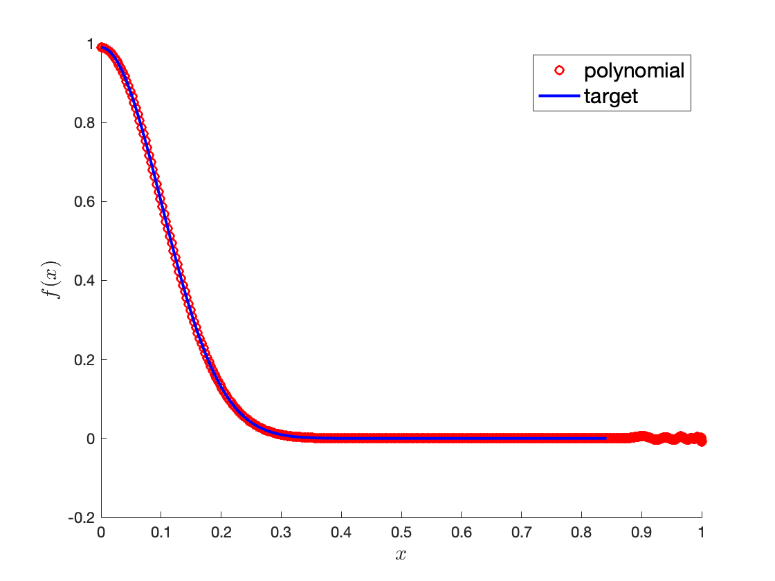
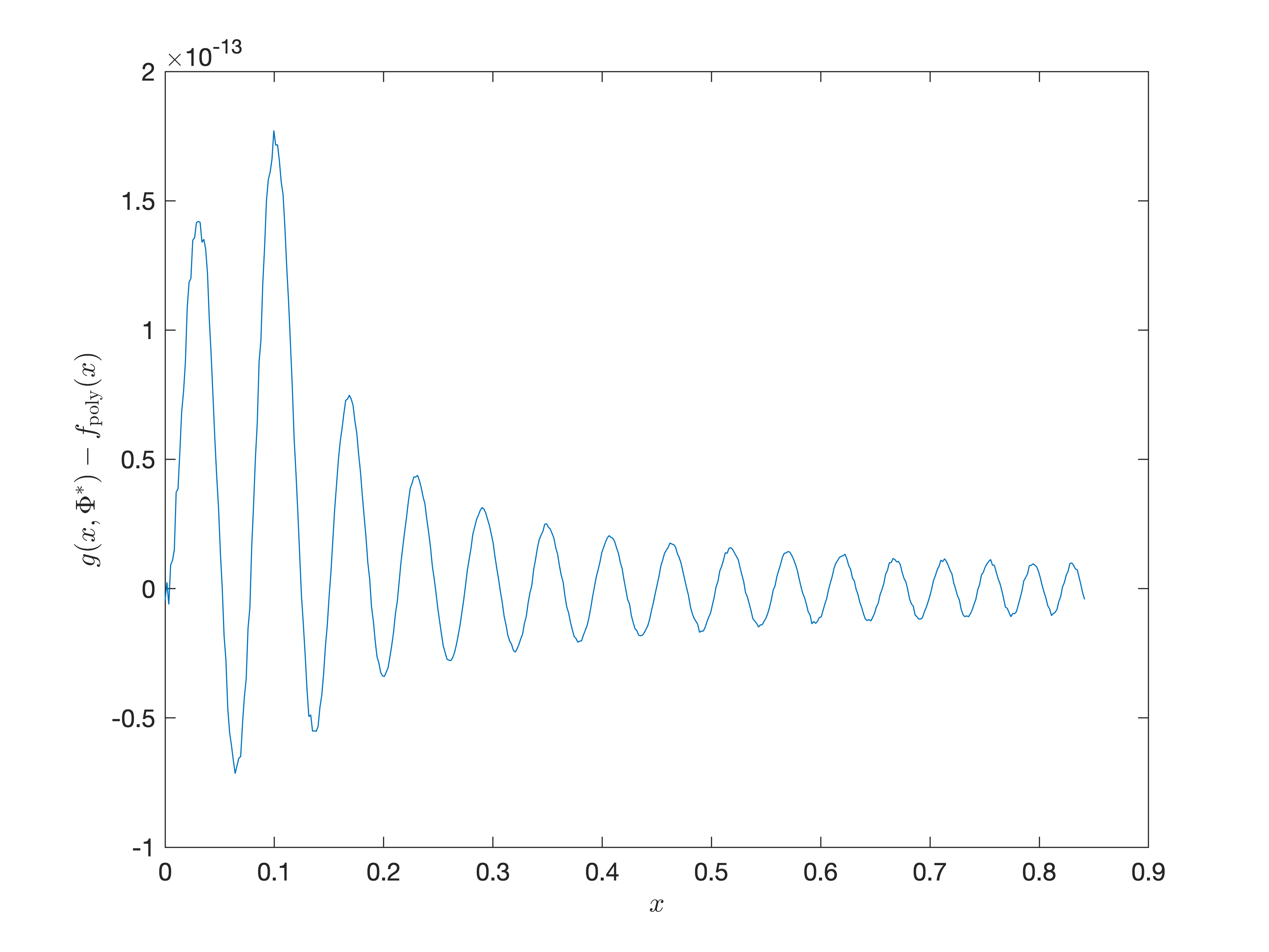
### Approximating the target function by polynomials

```matlab
coef_full=cvx_poly_coef(targ, deg, opts); 
parity = mod(deg, 2); 
% only keep coefficients with consistent parity
coef = coef_full(1+parity:2:end);
```

<div><figure><img src="https://40428858-files.gitbook.io/~/files/v0/b/gitbook-x-prod.appspot.com/o/spaces%2FznDlSgNqsJLx79OHu47P%2Fuploads%2FNLKVgCIjfxtJRWQMxyDi%2Fgaussian_state_polynomial.png?alt=media&#x26;token=e37e50e0-8ba4-4152-9c80-1772672602f3" alt=""><figcaption><p>Polynomial approximation of gaussian function</p></figcaption></figure> <figure><img src="https://40428858-files.gitbook.io/~/files/v0/b/gitbook-x-prod.appspot.com/o/spaces%2FznDlSgNqsJLx79OHu47P%2Fuploads%2FRglqHFtKkmkoMNqkP9YF%2Fgaussian_state_pointwise_error.png?alt=media&#x26;token=2df173ad-852d-4af7-bd47-388b77e27610" alt=""><figcaption><p>Polynomial approximation error</p></figcaption></figure></div>

### Solving phase factors by running the solver

```matlab
[phi_proc,out] = QSP_solver(coef,parity,opts);
```

### Verifying the solution

```matlab
xlist = linspace(0,sin(1),500)';
func = @(x) ChebyCoef2Func(x, coef, parity, true);
targ_value = targ(xlist);
func_value = func(xlist);
QSP_value = QSPGetEntry(xlist, phi_proc, out);
err= norm(QSP_value-func_value,Inf);
disp('The residual error is');
disp(err);

figure()
plot(xlist,QSP_value-func_value)
xlabel('$x$', 'Interpreter', 'latex')
ylabel('$g(x,\Phi^*)-f_\mathrm{poly}(x)$', 'Interpreter', 'latex')
```

<figure><img src="https://40428858-files.gitbook.io/~/files/v0/b/gitbook-x-prod.appspot.com/o/spaces%2FznDlSgNqsJLx79OHu47P%2Fuploads%2Fp0aTD0KRMDteMiZO6sw7%2Fgaussian_state_preparation.png?alt=media&#x26;token=0ed7bfd7-514b-462d-a042-ff436dd4a994" alt="" width="563"><figcaption><p>The point-wise error of the solved phase factors.</p></figcaption></figure>

### Reference

1. McArdle, S., Gilyén, A., & Berta, M. (2022). Quantum state preparation without coherent arithmetic. *arXiv preprint arXiv:2210.14892*.

<details>

<summary>Output of the code</summary>

```
norm error = 1.34851e-09
max of solution = 0.99
L-BFGS solver started 
iter          obj  stepsize des_ratio
   1  +1.1629e-02 +1.00e+00 +4.86e-01
   2  +8.0537e-03 +1.00e+00 +7.10e-01
   3  +3.8400e-03 +1.00e+00 +6.69e-01
   4  +1.6803e-03 +1.00e+00 +7.00e-01
   5  +6.2256e-04 +1.00e+00 +6.84e-01
   6  +2.1175e-04 +1.00e+00 +6.84e-01
   7  +6.3658e-05 +1.00e+00 +6.79e-01
   8  +1.6662e-05 +1.00e+00 +6.75e-01
   9  +9.0703e-06 +1.00e+00 +6.93e-01
  10  +4.0572e-06 +1.00e+00 +7.32e-01
iter          obj  stepsize des_ratio
  11  +1.3684e-06 +1.00e+00 +7.01e-01
  12  +4.1191e-07 +1.00e+00 +6.36e-01
  13  +1.6236e-07 +1.00e+00 +6.16e-01
  14  +6.8715e-08 +1.00e+00 +6.64e-01
  15  +2.1314e-08 +1.00e+00 +6.90e-01
  16  +1.1814e-08 +1.00e+00 +6.88e-01
  17  +1.5959e-09 +1.00e+00 +6.20e-01
  18  +7.3575e-11 +1.00e+00 +5.69e-01
  19  +2.3390e-12 +1.00e+00 +5.55e-01
  20  +3.8866e-13 +1.00e+00 +6.20e-01
iter          obj  stepsize des_ratio
  21  +1.5834e-14 +1.00e+00 +5.60e-01
  22  +2.1621e-16 +1.00e+00 +5.45e-01
  23  +6.4336e-19 +1.00e+00 +5.19e-01
  24  +5.0662e-21 +1.00e+00 +5.23e-01
  25  +2.1126e-22 +1.00e+00 +5.68e-01
  26  +1.1727e-24 +1.00e+00 +5.29e-01
  27  +1.1873e-26 +1.00e+00 +5.33e-01
Stop criteria satisfied.
The residual error is
   1.7719e-13
```

</details>
